Look here for the syllabus and more information.
You can also have a look at a previous semester's (2005) web site of mine for the same course.
Main lectures: MWF 14:05 - 14:55, in Skiles 202.
My office hours are: Thu 10-12 in my office (Skiles 133).
You're also welcome to ask me questions any time you see me, anywhere.
Recitation sessions: TTh 14:05-14:55 in Skiles 202 (instructor Daniel Tiefa)
Dan's office hours are TBA.
There will be quizzes each Thursday (except for the first one) for the last 15 minutes of the session. One problem will be asked among those (or very much resembling one of those) that were assigned as homework.
The quizzes are worth 20% of the grade (the two smallest quiz scores will be discounted for each of you), each of the two midterms (Feb 9 and March 14) is worth another 20% and the final is worth 40%.
We covered §13.1.
We saw examples of functions of a real variable whose values are 2D or 3D vectors.
We defined the limit
HW problems: §13.1: 1, 2, 15, 16, 21, 22, 27, 28, 39, 41.
For the first week only, my office hours will be held on Friday, 3-5.
We saw how to compute the derivatives of vector valued functions which have been
made by piecing together, in various ways, other functions. For example, we saw that
if ![]() is a scalar function and
is a scalar function and ![]() is a vector function then the derivative
of the function
is a vector function then the derivative
of the function ![]() which is defined by
which is defined by
HW problems: §13.2: 1, 2, 4, 6, 7, 9, 11, 17, 18, 21, 22, 27, 29, 32.
The first midterm exam will take place on Fri, Feb 9, during our regular meeting and in the same place.
The second midterm will take place on Wed, Mar 14, also during our regular meeting and in the same place.
We saw a few examples of vector-valued functions viewed as parametrizations of
curves in space. We saw that when ![]() traverses a curve
traverses a curve ![]() then
then
![]() is a tangent vector
of
is a tangent vector
of ![]() at point
at point ![]() , and solved some problems which
asked geometric questions about curves that had been described in parametric
form.
We also saw how to find the intersection points of two curves that have
been given to us in parametrized form. One must be careful in this problem not
to use the same name of the parameter for both curves.
, and solved some problems which
asked geometric questions about curves that had been described in parametric
form.
We also saw how to find the intersection points of two curves that have
been given to us in parametrized form. One must be careful in this problem not
to use the same name of the parameter for both curves.
Some of the problems listed below you cannot solve without reading the rest of §13.3 (we will cover this on Wednesday).
HW problems: §13.3: 1-4, 9, 14, 15, 18, 35-38.
We finished §13.3: talked about the unit tangent vector ![]() to a curve at point
to a curve at point ![]() and the principal normal vector
and the principal normal vector ![]() as well as the osculating plane they define. We computed
an example.
as well as the osculating plane they define. We computed
an example.
Then we saw how to calculate the length of a curve parametrized by the vector function ![]() ,
for
,
for ![]() . We computed some examples and also saw by example that the formula we gave
for arc-length does not depend on the parametrization of the curve. That is we took two different
paraetrizations of a specific curve (a circle, actually) and used our length formula with
both of these parametrizations and we got the same result, as we should.
. We computed some examples and also saw by example that the formula we gave
for arc-length does not depend on the parametrization of the curve. That is we took two different
paraetrizations of a specific curve (a circle, actually) and used our length formula with
both of these parametrizations and we got the same result, as we should.
HW problems: §13.4: 1-4, 8, 9, 17, 23.
My office hours tommorrow, Thursday Jan 18, will be held from 9-11 (not 10-12) as I want to go to a lecture at 11 (this change may become permanent).
If any of your planned to see me from 11-12, please send me a message to set up an appointment (but not on Thursday).
We covered the part of §13.5 that concerns plane curves and their curvature. We saw how to
reparametrize a curve which has been given to us in parametric form ![]() in such a way that
the parameter is now
in such a way that
the parameter is now ![]() the arc-length along the curve. This parametrization has the property,
which characterizes it, that the velocity vector has constant magnitude equal to
the arc-length along the curve. This parametrization has the property,
which characterizes it, that the velocity vector has constant magnitude equal to ![]() .
The curvature of a plane curve is defined as the derivative with respect to
.
The curvature of a plane curve is defined as the derivative with respect to ![]() of the angle formed
by the tangent line to the curve and the
of the angle formed
by the tangent line to the curve and the ![]() -axis, in absolute value. (This definition will have to
be amended next time in order to define the curvature of space curves.) We then saw formulas
that allow us to calculate the curvature given the parametrization of the curve. We applied these
formulas to several examples. Finally we defined the radius of curvature and the center of curvature.
-axis, in absolute value. (This definition will have to
be amended next time in order to define the curvature of space curves.) We then saw formulas
that allow us to calculate the curvature given the parametrization of the curve. We applied these
formulas to several examples. Finally we defined the radius of curvature and the center of curvature.
Of the following problems, do now those that concern plane curves, and leave those about space curves for after having finished §13.5.
HW Problems: §13.5: 1, 2, 5, 6, 10, 13, 14, 21, 22, 41, 42, 58.
We saw how one defines the curvature ![]() of space curves (curves which are not known
to be contained in a plane) and computed some examples.
of space curves (curves which are not known
to be contained in a plane) and computed some examples.
We also saw that acceleration of a particle moving along a curve ![]() , that is
the vector
, that is
the vector
Do the problems of §13.5, listed above, which you could not do before today's lecture.
We covered §13.6. We saw how to apply some of the things we've seen so far to problems of Mechanics (motion of particles under certain forces). In particular, we proved Kepler's 2nd law which states that if a particle is moving under the influence of central force (force parallel to the location vector) then its location vector sweeps out equal areas in equal times.
We did not have time to cover the subsection on initial value problems. Please go over Examples 3 and 4 on p. 809 and 810.
HW Problems: §13.6: 1-4, 8, 9, 11, 14, 15.
We talked a little about how to solve initial value problems of the second order such as those that arise from Newton's equation in kinematics (read §13.6).
Then we moved on to §14.1 and talked about real-valued functions of two or three variables
HW Problems: §14.1: 1-10, 35, 37, 39.
We first remembered what kind of curves in the plane have an equation ![]() which is
a polynomial in
which is
a polynomial in ![]() and
and ![]() of degree at most
of degree at most ![]() , a quadratic equation. These are the so-called
conic sections: ellipse, hyperbola, parabola, straight line, a pair of straight lines or
a single point. Next we wrote down the general quadratic equation in three variables
, a quadratic equation. These are the so-called
conic sections: ellipse, hyperbola, parabola, straight line, a pair of straight lines or
a single point. Next we wrote down the general quadratic equation in three variables ![]() , that is
an arbitrary polynomial in these variables whose degree is at most
, that is
an arbitrary polynomial in these variables whose degree is at most ![]() . The case now are many more
and I am not asking that you memorize the entire list in your book (§14.2) but that you learn,
as we did in class, how to figure out the shape of a given surface, whose equation you're given, by
cleverly fixing some of the variable to appropriate values (in your book these are called intercepts
and traces), and also by taking advantage of the symmetries of the equation. Do learn the few examples
we did in class.
. The case now are many more
and I am not asking that you memorize the entire list in your book (§14.2) but that you learn,
as we did in class, how to figure out the shape of a given surface, whose equation you're given, by
cleverly fixing some of the variable to appropriate values (in your book these are called intercepts
and traces), and also by taking advantage of the symmetries of the equation. Do learn the few examples
we did in class.
HW Problems: §14.2: 2, 4, 10, 12, 20, 22, 26, 40, 43.
A student note taker is needed in this course to take notes for a student with a disability. The note taker will be paid a stipend for this assignment. Skills needed are the ability to take accurate, legible, and organized notes and a commitment to attend every lecture. If interested, please contact Tina Allen via office phone at 404-894-2563 or via email at notetaker@vpss.gatech.edu as soon as possible. Be sure to indicate the Professor's name, time, day and course number/ section in the subject line of the announcement.
We saw how to present geometric information about a function ![]() or
or ![]() (or its
graph, representable by the equation
(or its
graph, representable by the equation ![]() or
or ![]() ) by drawing its level curves
for two-variable functions, i.e. the curves whose equation is given by
) by drawing its level curves
for two-variable functions, i.e. the curves whose equation is given by ![]() for
various values of
for
various values of ![]() , or its level surfaces (three-variable case) which are the surfaces
representable by the equation
, or its level surfaces (three-variable case) which are the surfaces
representable by the equation
![]() , again for various values of
, again for various values of ![]() .
.
HW Problems: §14.3: 4, 5, 8, 14, 19, 20, 21, 25, 28.
Next we saw how one defines the partial derivatives (with respect to each of the variables) of functions of more than one variable, and saw how to compute some examples by treating all variables but the one we're differentiating with as constants.
My apologies to those of you (if any) who came to my office hours Thursday. I entirely forgot.
I will be in my office from 4-5 tomorrow Friday.
Mihalis
We finished §14.4, by giving more examples of how to compute the partial derivatives
of functions of several variables and by talking about the geometric significance of
the partial derivatives of a function ![]() .
.
HW Problems: §14.4: 1-10, 23, 41, 53.
We then started speaking about §14.5. We defined the ![]() -neighborhood (and deleted neighborhood)
of a point
-neighborhood (and deleted neighborhood)
of a point
![]() , where
, where ![]() . We also defined the concept
of an open set
. We also defined the concept
of an open set
![]() and saw, as an example, that the upper half plane
and saw, as an example, that the upper half plane
![]() :
:
You can find a practice exam (for 50 min) here in PDF.
We defined what closed sets are (the complements of open) sets as well as what the interior points of a set are and its boundary points. We saw several examples, both in dimension 2 as well as in dimension 1.
HW Problems: §14.5: 1-20.
For the first test (this Friday, in class) you are expected to know all that has been taught to you by today (Monday). Please come early so as to start on 14:05 sharp.
There will be a quiz on Thursday as usual.
We went over the practice exam and aswered some questions.
We had our first test. Here are the problems.
Solution:
Velocity:
![]() .
.
Speed:
![]() .
.
Force:
![]() .
.
Solution:
(a)
![]() .
.
(b) For a vector to be parallel to the ![]() -plane means that its
-plane means that its ![]() -coordinate is
-coordinate is ![]() . This
happens for the first time at
. This
happens for the first time at ![]() . At that moment the velocity
vector is
. At that moment the velocity
vector is
![]() . A parametrization of the tangent line (which goes through
the point
. A parametrization of the tangent line (which goes through
the point
![]() and has the direction of the vector
and has the direction of the vector ![]() is
is
Solution:
(a) The argument of the function ![]() must be positive, hence the domain is
must be positive, hence the domain is
Solution:
(a) This is the region where ![]() and
and ![]() have the same sign or some of them is zero. This is the
first and third quadrant of the plane, together with the
have the same sign or some of them is zero. This is the
first and third quadrant of the plane, together with the ![]() - and
- and ![]() -axes.
-axes.
Any point of that set which is not on the axes is an interior point as one can draw a disk centered at it which is entirely in the set. Any point on the axes is not an interior point as any disk around such a point will contain points outside the first and third quadrant.
For this reason all points of the axes are boundary points. There are no other boundary points as any point
inside a quadrant and not on an axis will have a small disk around it which contains either only points of
the set or of its complement and not from both.
(b) The only difference of this shape from that of (a) is that the ![]() - and
- and ![]() -axes are not part of
the set now. However the set of interior points and the set of the boundary points remains the same
as that of (a). (In this case the set of boundary points, namely the two axes, is not part of the set itself.)
-axes are not part of
the set now. However the set of interior points and the set of the boundary points remains the same
as that of (a). (In this case the set of boundary points, namely the two axes, is not part of the set itself.)
We defined formally what the limit of a two-variable function is when
![]() ,
and when a function is continuous at a point
,
and when a function is continuous at a point ![]() .
We calculated the limits using the definition for some very simple functions.
.
We calculated the limits using the definition for some very simple functions.
We also saw examples of functions of two variables which exhibit strange behaviour, by one variable standards. For example we saw a function which is everywhere continuous with respect to each of the variables and has everywhere partial derivatives, yet is not continuous at (0,0).
HW Problems: §14.6: 1-5, 21, 23, 24, 26, 27.
You can find your grade here in PDF.
We defined what it means for a function of many variables to be differentiable at a point ![]() ,and also defined the gradient of a differentiable function
,and also defined the gradient of a differentiable function ![]() at
at ![]() , as the only
vector
, as the only
vector ![]() that makes the following true:
that makes the following true:
See, for example, this page for the big-O and little-o notation that we talked about today.
HW Problems §15.1: 12-16, 33-37, 39, 40.
We talked about the concept of directional derivatives and how to compute them using the gradient of a function. Also saw that the direction of the gradient is the direction of maximum rate of increase of a function. Saw several examples.
HW Problems §15.2: 11-14, 23-26, 40, 41.
We went over the Mean Value Theorem for scalar functions of one variable, and used it to prove the mean value theorem for scalar functions of a vector variable. We remarked that the Mean Value Theorem is not true for vector valued functions. We saw some consequences of the MVT: if two functions have the same gradient in a connected open set then they differ by a constant.
Next we reviewed the chain rule for functions of one variable and saw the form it takes for the composition of a scalar function of a vector variable with a vector valued function of one variable. We saw how to construct the dependency diagram when we have many quantities that depend on others, and use it to derive the appropriate chain rule.
Please read from §15.3 about implicit differentiation.
HW Problems §15.3: 1, 3, 4, 6-8, 17, 18, 25, 27, 29, 30, 36, 58.
We pointed out that
![]() is a normal vector to the curve (or surface)
is a normal vector to the curve (or surface)
![]() ,
, ![]() a constant. We used this to compute normal and tangent vectors
to curves and surfaces amd also angles between curves and surfaces. These angles
are defined to be the corresponding angles between their tangent objects at
the intersection. For example, if we are seeking the angle between a curve and a surface
which intersect at a point
a constant. We used this to compute normal and tangent vectors
to curves and surfaces amd also angles between curves and surfaces. These angles
are defined to be the corresponding angles between their tangent objects at
the intersection. For example, if we are seeking the angle between a curve and a surface
which intersect at a point ![]() we must measure the angle between a tangent vector of the curve at
we must measure the angle between a tangent vector of the curve at ![]() and the
tangent plane to the surface at
and the
tangent plane to the surface at ![]() . This is most easily measured by first finding
the angle between the tangent to the curve and the normal to the tangent plane, and then
subtracting that angle from
. This is most easily measured by first finding
the angle between the tangent to the curve and the normal to the tangent plane, and then
subtracting that angle from ![]() .
.
HW Problems §15.4: 1, 2, 10, 11, 19, 20, 26, 27, 28, 34, 36.
We saw what is the analogue in two variables of the criteria, involving first and second derivatives, that we know for deciding where a function's local maxima and minima are. The first stage of the method is to locate the points where the function's gradient vanishes. Each of those points is then checked using higher order partial derivatives of the function at that point in order to decide if there is a local extremum at that point or if it is a saddle point.
HW Problems §15.5: 1, 2, 5-8, 25, 26.
We saw how to find the (global) minima or maxima of a function of two variables defined in a closed and bounded domain. We have to find the critical points in the interior of the domain and then parametrize our boundary, which gives rise to a function of one variable corresponding to our function being evaluated on the boundary. This one-variable function we extremize (find its extrema) separately. The extrema of this one-variable function along with the critical points in the interior are then compared in the value of the function at them to find the global extrema.
HW Problems §15.6: 1-6, 19-22, 27.
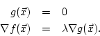
We talked about the problem of finding the minimum or maximum of a function ![]() when
when
![]() is not free to take any values in the domain of definition of
is not free to take any values in the domain of definition of ![]() but it has to satisfy
some condition, which is usually given in the form
but it has to satisfy
some condition, which is usually given in the form ![]() .
Sometimes one can solve
.
Sometimes one can solve ![]() for one of the variables in
for one of the variables in ![]() and substitute the
resulting expression in
and substitute the
resulting expression in ![]() thus getting a problem of ordinary function extremization
without side conditions and in one variable less. We saw two such examples but this
method is most often inapplicable as it is not easy to solve
thus getting a problem of ordinary function extremization
without side conditions and in one variable less. We saw two such examples but this
method is most often inapplicable as it is not easy to solve ![]() for one of the variables,especially if
for one of the variables,especially if ![]() is a three-component vector and
is a three-component vector and ![]() is non-linear.
Even if possible the resulting expression for
is non-linear.
Even if possible the resulting expression for ![]() may be too complicated to work with.
may be too complicated to work with.
We then saw the method of Lagrange (or Lagrange multipliers as it is commonly known),
which allows one to solve the above problem by solving a, generally non-linear,
system of equations in the unknowns ![]() and
and ![]() , the latter being a auxiliary
variable which is not used except to help find the values of
, the latter being a auxiliary
variable which is not used except to help find the values of ![]() .
The system of equations is
.
The system of equations is
HW Problems §15.7: 1-4, 13, 15, 18, 19, 21, 23.
We gave some more examples of the method of Lagrange multipliers and saw how it applies to the case of a function of three variable subject to two conditions.
We also saw that there is a way to avoid introducing the Lagrange multiplier (the ![]() variable, which we throw away after solving the system of equations). This can
be done by checking the parallelism between the two fectors
variable, which we throw away after solving the system of equations). This can
be done by checking the parallelism between the two fectors ![]() and
and
![]() (the gradients of the function to be optimized and the constraint function) by checking the
equation
(the gradients of the function to be optimized and the constraint function) by checking the
equation
The answer is that the vector equation
![]() is really only two
equations. If one writes it out (using the determinant form) one notices immediately
that any of the resulting three equations can be obtained from the other two, so one can throw
away any one of them (but only one) without changing the solutions to our system.
Now it is clear that we have three equations in three unknowns.
is really only two
equations. If one writes it out (using the determinant form) one notices immediately
that any of the resulting three equations can be obtained from the other two, so one can throw
away any one of them (but only one) without changing the solutions to our system.
Now it is clear that we have three equations in three unknowns.
We saw how to use the summation sign and iterated (multiple) summation sign via several examples. We also evaluated several simple sums.
HW Problems §16.1: 1-4, 13-17.
You can find a practice exam (for the 50 min 2nd midterm) here in PDF.
Note Taker Announcement:
A student note taker is needed in this course to take notes for a student with a disability. The note taker will be paid a stipend for this assignment. Skills needed are the ability to take accurate, legible, and organized notes and a commitment to attend every lecture. If interested, please contact Christina Bibbs at notetaker@vpss.gatech.edu, and be sure to indicate the Professors name, time, day and course number in the subject line of your email. Thank you so much for your willingness to assist our office in this process. Please contact our office if we can be of any assistance.
We defined the integral of a function ![]() over a rectangle
over a rectangle ![]() via
lower and upper sums corresponding to partitions of
via
lower and upper sums corresponding to partitions of ![]() . We
evaluated, using the definition, only some simple integrals.
. We
evaluated, using the definition, only some simple integrals.
HW Problems §16.2: 1, 2, 6, 7, 10, 11.
We stated the Mean Value Theorem for double integrals over connected domains (§16.2).
When a domain is such that all its intersections with lines parallel to the ![]() -axis are intervals,
and the set of
-axis are intervals,
and the set of ![]() -values used in the domain consititute an interval the domain is called of Type I
(and of Type II if the same properties hold with
-values used in the domain consititute an interval the domain is called of Type I
(and of Type II if the same properties hold with ![]() and
and ![]() reversed). For such a domain
we saw how to evaluate a double integral of a function as a single integral whose function to be integrated
is an integral itself.
reversed). For such a domain
we saw how to evaluate a double integral of a function as a single integral whose function to be integrated
is an integral itself.
HW Pproblems §16.3: 1-6, 13, 14, 33, 34, 43, 46.
We did not cover any new material. Instead we went over the practice exam, in preparation for Wednesday's exam.
We had our second test. Here are the problems:
Solution:
Suppose the vertex of the box lying in the first octant has coordinates ![]() , with
, with
![]() . It follows that the volume of the box is
. It follows that the volume of the box is
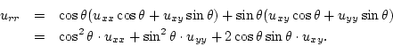
Solution: We have
Solution:
The surface is a level surface of the function
Your formula for ![]() may not involve partial derivatives of
may not involve partial derivatives of ![]() with respect to
with respect to ![]() or
or ![]() .
.
Solution:
We have
![]() and
and
![]() .
By the chain rule we get
.
By the chain rule we get
You may find them here in PDF.
We went through the problems that were on the last test and their solutions.
We saw how to evaluate a double integral using polar coordinates. The first task is to find
the domain ![]() in the
in the ![]() -plane which corresponds to the given domain
-plane which corresponds to the given domain
![]() (in the
(in the ![]() -plane). For example, if
-plane). For example, if ![]() is the unit disk in the cartesian plane
(the
is the unit disk in the cartesian plane
(the ![]() -plane) then
-plane) then ![]() is a rectangle in the
is a rectangle in the ![]() -plane defined by
-plane defined by
Please read by yourselves the evaluation of
![]() from the
end of §16.4. This is a very important integral in all mathematics and especially its applications
to science and engineering.
from the
end of §16.4. This is a very important integral in all mathematics and especially its applications
to science and engineering.
HW Problems §16.4: 1, 2, 5, 6, 9, 10, 17-20, 23, 24.
We covered a couple more examples from §16.4 and proved the identity
We covered some of the examples in §16.5. We saw how to compute the mass of a two-dimensional domain (a ``plate'') with variable density, and also how to compute its center of mass. We also saw the definition of the moment of inertia of a plate (with variable density) rotating around a line or point. We evaluated some relevant double integrals.
HW Problems §16.5: 1-4, 11, 12, 14, 17, 25.
We saw briefly how triple integrals are defined (in a completely analogous way to double integrals, so we did not insist much on §16.6) and proceeded to evaluate some triple integrals by repeated integration.
HW Problems §16.7: 3-6, 11, 14-16, 21-22.
We showed how to compute a triple integral in cylindrical coordinates.
HW Problems §16.8: 1-8, 11, 12, 17, 18, 25, 26.
We introduced the spherical coordinate system and how to use it for evaluation
of triple integrals.
We saw several examples of how to transform the domain of integration from cartesian
to spherical coordinates and carry out the integration in spherical coordinates (the form
![]() becomes now
becomes now
![]() ).
).
HW Problems §16.9: 1-4, 9-14, 16, 19, 20, 24, 26, 27.
We saw the general procedure for evaluating a multiple (double or triple) integral
over a domain ![]() after first doing a change of variables. This is essentially
a way of parametrizing
after first doing a change of variables. This is essentially
a way of parametrizing ![]() using two or three variables (depending on the whether the
domain
using two or three variables (depending on the whether the
domain ![]() is in the plane or space) which run over a more convenient
domain
is in the plane or space) which run over a more convenient
domain ![]() . We say how to do this when
. We say how to do this when ![]() is a parallelogram (and we got a parametrization
with paramaters
is a parallelogram (and we got a parametrization
with paramaters ![]() and
and ![]() running through the rectangle
running through the rectangle
![]() )
and also in some other cases.
We also saw that the form
)
and also in some other cases.
We also saw that the form ![]() transforms into the form
transforms into the form
![]() (and similarly in three dimensions), where
(and similarly in three dimensions), where ![]() is the so-called
Jacobian determinant, which can be computed from the functions
is the so-called
Jacobian determinant, which can be computed from the functions ![]() and
and ![]() .
.
HW Problems §16.10: 1-2, 8-10, 12-14, 19, 20, 27, 29.
We defined the line integrals of a vector field
![]() along a curve
along a curve ![]() given parametrically by
given parametrically by ![]() ,
, ![]() ,
as the expression
,
as the expression
HW Problems §17.1: 1-4, 7, 15, 16, 20, 21, 23, 25, 28-30.
This says that if a vector field ![]() is a gradient field, then a line integral of that
along a curve
is a gradient field, then a line integral of that
along a curve ![]() equals the value of
equals the value of ![]() (where
(where
![]() ) equals
) equals
![]() where
where ![]() and
and ![]() are the endpoints of
are the endpoints of ![]() . This is true in two and three dimensions,
and, in two dimensions, in order to decide if
. This is true in two and three dimensions,
and, in two dimensions, in order to decide if ![]() is a gradient field we need to verify
that
is a gradient field we need to verify
that ![]() when the domain
when the domain ![]() , where
, where ![]() is defined, is simply connected (i.e. connected
and with no ``holes'').
is defined, is simply connected (i.e. connected
and with no ``holes'').
HW Problems §17.2: 1-4, 12, 13, 22, 24-26, 28.
My office hours tomorrow, April 12, will last only until 11am.
We discussed kinetic energy and why its change is due to the work is done by the force field on the particle. Also we talked about conservative (gradient) fields and the potential function.
HW Problems §17.3: 1-3, 6, 7, 8.
We saw an alternative way of writing the line integral
![]() as
as
![]() , where
, where
![]() .
We also saw the line integral w.r.t. arc-length, denoted by
.
We also saw the line integral w.r.t. arc-length, denoted by ![]() , where
, where
![]() is a scalar function.
is a scalar function.
HW Problems §17.4: 2, 3, 5, 17, 18, 26, 27, 29, 30, 32, 36.
We stated Green's theorem. This expresses a line integral along a closed curve as a double integral over the interior of that curve. We proved this in the case when the domain if of Type I and of Type II and showed how one proves this if the domain is more general by cutting up the domain into a finite number of non-overlapping parts each of which is of both Type I and II. We also explained how to parametrize the boundary of a domain if that is not simply connected or even not connected (walk along the boundary in such a way that the domain is always on your left).
HW Problems §17.5: 1, 2, 5, 6, 18-20, 26, 28, 30, 31.
We saw how to apply Green's formula to derive a formula for the area of a polygonal region
that has been described to us by the coordinates of its vertices. We also saw how to find an analogous
formula for the centroid of the polygon and for the volume
of the solid that arises if we rotate a polygonal region
(which is part of the right half plane
![]() ) about the
) about the ![]() -axis.
-axis.
We saw how to calculate the area of a surface which has been given to us in parametric form.
HW Problems §17.6: 1, 2, 5, 6, 15, 16, 17, 22, 23, 35, 36.
You may find it here in PDF.
I answered various questions of the students.
We went through the practice final exam that was distributed on Wednesday.
It will take place in Skiles 202 (lecture room), on Friday May 4, from 11:30 to 14:20.
We had our final exam. Here are the problems:
Hint: Use the normal vectors to ![]() and
and ![]() at
at ![]() .
.
Hint: Do not use Green's theorem.
You may find them here.
I will be in my office on Sunday May 6, from 6 to 7pm, in case somebody wants to see an exam paper. After that the grades will be finalized.
Mon May 7 20:15:18 EDT 2007: There had been an error in the software that computed your numerical scores, which had as an effect that the quizzes were not counted (and possibly other effects). This error has now been corrected (I hope) and your numerical grades are now correctly computed (please, check yours, and let me know if you believe there is a numerical error in your posted numerical grade).
Some letter grades have inevitably been changed as the landscape changed, most of them for the better I believe, but not all.
I will enter the corrected grades into the system tomorrow but the process is slow and the changes may not show up online for several days.
I apologize for this mistake. I wish one of you had checked the numbers concerning him/her but, amazingly, no one did (at least, no one notified me of the discrepancy). Neither did I until today when I realized the error.