Look here for the syllabus and more information.
MWF 15:05 - 15:55, in Skiles 271.
My office hours are: 9-11 Tuesdays, in my office (Skiles 209). You're also welcome to ask me questions any time you see me, anywhere.
Two midterm exams will be given and a final. If the three grades are ![]() ,
, ![]() and
and ![]() then
the final grade for the class will be given by
then
the final grade for the class will be given by
Homework will be assigned but will not be normally collected. Do it to be adequately prepared for the tests, as the problems on these will be small variations of those on the homework assignments.
We went over §13.1, and talked about what is a vector valued function of
a real variable. We saw how the properties of limit (as ![]() ) are defined,
the concept of continuity, differentiability and integration.
All of these properties and quantities can be defined either with direct reference
to the vector values of the function or with reference to the components
of the function.
) are defined,
the concept of continuity, differentiability and integration.
All of these properties and quantities can be defined either with direct reference
to the vector values of the function or with reference to the components
of the function.
Look at problems §13.1: 39, 40, 43, 46, 51, 53, 55, 57.
We covered §13.2. We saw that differentiation of vector valued functions obeys the expected rules, very similar or identical to those obeyed by scalar-valued functions. We did problems §13.2: 28, 29, 31, 33.
Look at problems §13.2: 35, 36.
We covered §13.3. The main things we learned about is the tangent line and the tangent vector on a curve at one of its points and also the normal vector to it. Together the tangent and normal vector to a curve define the osculating plane, which is a plane that goes through a point on the curve and contains the tangent line and the normal vector.
Forgot to mention it in class but do look at problems §13.3: 1, 2, 9, 11, 14, 18, 33, 35, 36, 37, 45.
In §13.4 we saw how to define and calculate the length of a curve which is given to us in parametric form. The answer is that we integrate over time (or whatever our paramater is called, but we think about it always as time) the speed of the motion, that is the magnitude of the velocity vector (derivative of the location vector).
We calculated several examples.
Look at problems §13.4: 7, 9, 17, 21, 23 (this last one has to do with the so-called arc-length parametrization of a given curve, so pay special attention to it).
We defined the curvature of a plane curve as the rate of change of the angle
formed by the tangent and the ![]() -axis as we are moving along the curve at unit speed.
We then found how to calculate the curvature for a curve that is the graph of a function
and then for a curve which is given to us in parametric form.
We also defined the radius of curvature and the center of curvature of
a curve at a given point (provided the curvature there does not vanish).
Then we proved the formula
-axis as we are moving along the curve at unit speed.
We then found how to calculate the curvature for a curve that is the graph of a function
and then for a curve which is given to us in parametric form.
We also defined the radius of curvature and the center of curvature of
a curve at a given point (provided the curvature there does not vanish).
Then we proved the formula

Look at problems §13.5: 2, 5, 6, 10, 13, 14,21, 22, 41, 42, 58.
We completed our discussion of curvature for palne curves and evaluated it in some examples. Then we talked about mechanics and we expressed (but not proved) Theorem 13.6.7 in your book and talked about its qualitative consequences for planetary motion.
We proved Kepler's second law (that a particle moving in a central force field
is always executing a planar motion and that its location vector sweeps out
equal areas in equal times). We also formulated Kepler's first and third law.
We solved an initial value problem, where the force field is given and also the
initial location and velocity of the particle and the motion of the particle
(function ![]() ) is to be determined.
) is to be determined.
Look at problems §13.6: 2, 3, 5, 7, 8, 15.
It was also announced that your first test will come after we complete Chapter 14 and the material covered will be Chapters 13 and 14.
We proved Kepler's 1st law, namely that the planets are moving in elliptical orbits with the sun at a focus. We carried out the proof to the point where the equation of an ellipse was determined in polcar coordinates.
No problems for homework from this session.
Do the following problems in an hour with closed books (no calculators will be needed). In any test you write for this class you'll have to show all your work.
We covered §14.1, and we talked about functions which depend on several variables (typically
two or three, but that's not necessary) and how to find their domain (given a formula
for them) and their range. We also talked about the general quadric surface in
![]() which is a surface defined by a polynomial equation in three variables
which is a surface defined by a polynomial equation in three variables ![]() such that
the degree of each monomial is at most two (the general quadratic). We described the ellipsoid,
which is one of them.
such that
the degree of each monomial is at most two (the general quadratic). We described the ellipsoid,
which is one of them.
Look at problems §14.1: 1-10, 35-37, 39.
After a brief reminder of the several different kinds of curves in the plane
that have a quadratic equation describing them (ellipses, hyperbolas and parabolas)
we described some of the different types of surfaces that a quadratic
equation in ![]() and
and ![]() can represent. We did not give an exhaustive list
but worked with 3-4 of those kinds and tried to figure out how they
look like by studying their intersection with some specific planes. It is this skill
that I want you to learn from §14.2, not a list of surfaces.
can represent. We did not give an exhaustive list
but worked with 3-4 of those kinds and tried to figure out how they
look like by studying their intersection with some specific planes. It is this skill
that I want you to learn from §14.2, not a list of surfaces.
Do problems §14.2: 1-5, 10, 22, 24, 26, 39, 40, 43.
The first test will be held on W 9/22/04, during the regular meeting time. You should know the material in §13 and §14. Books will be closed. (But see §4.12.1.)
We talked about graphs of functions and how to visualize them by drawing their level curves (§14.3).
Do problems §14.3: 4, 5, 8, 14, 20, 21, 25, 28.
We also defined the partial derivatives of functions of several variables and calculated soem examples.
Please let me know in class Monday what your preferences are regarding when the first test will be administered.
We went again over the concept of partial derivatives, how to calculate them, and talked about their geometrical interpretation, mainly through problem 46 (§14.4) of your book.
Do problems §14.4: 1-10, 23, 24, 41, 53.
The first test will be held on F 9/24/04, during the regular meeting time. You should know the material in §13 and §14. Books will be closed. Please disregard the previous Announcement of §4.10.1.
The change has been asked by the class.
We covered the material in §14.5: what is a neighborhood of a point, which points of a set are called interior points, which are boundary points, which sets are called open and which closed. We gave several examples.
Do problems §14.5: 1-20.
We gave some more examples and general statements about open and closed sets.
We defined what it means for a function ![]() to have a limit as
to have a limit as
![]() ,
and we observed, through examples, that the situation is much more subtle that
with functions of one variable.
,
and we observed, through examples, that the situation is much more subtle that
with functions of one variable.
We saw again examples of functions of two variables which exhibit strange behaviour, by one variable standards. For example we saw a function which is everywhere continuous with respect to each of the variables and has everywhere partial derivatives, yet is not continuous at (0,0).
We saw (without proof) conditions that guarantee that the mixed partial derivatives of a function are equal.
Do problems §14.6: 1-5, 21, 23, 24, 26, 27.
On Wednesday we will review chapters 13 and 14. Please come armed with questions you want to ask.
Do the following problems in an hour with closed books (no calculators will be needed). In any test you write for this class you'll have to show all your work.
We had a review session for Chapters 13 and 14. On Friday we write our first test on these two chapters.
Today we had our first test. The problems were the following:
You can find the results of the first test here.
The most important comment I have to make is the almost complete and universal failure to do reasonably on the last problem.
If your score is less than 20 you should start working much harder on this class.
We defined what it means for a function of many variables to be differentiable at a point ![]() ,
and also defined the gradient of a differentiable function
,
and also defined the gradient of a differentiable function ![]() at
at ![]() , as the only
vector
, as the only
vector ![]() that makes the following true:
that makes the following true:
Do problems §15.1: 12-16, 33-37, 39, 40.
Most likely I will not be able to be in my office tomorrow T, 9/28/04. Please
schedule an appointment with me if you'd like to see me, or drop by at any other time.
This announcement is cancelled. Office hours wil be held as usual.
We talked about the concept of directional derivatives and how to compute them using the gradient of a function. Also saw that the direction of the gradient is the direction of maximum rate of increase of a function. Saw several examples.
Do problems §15.2: 11-14, 23-26, 40, 41.
We went over the Mean Value Theorem for scalar functions of one variable, and used it to prove the mean value theorem for scalar functions of a vector variable. We remarked that the Mean Value Theorem is not true for vector valued functions. We saw some consequences of the MVT: if two functions have the same gradient in a connect set then they differ by a constant.
Next we reviewed the chain rule for functions of one variable and saw teh form it takes for the composition of a scalar function of a vector variable with a vector valued function of one variable.
We completed our discussion of the various chain rules and saw how to differentiate functions defined implicitly.
Do problems §15.3: 1, 3, 4, 6-8, 17, 18, 25, 27, 29, 30, 36, 58.
We pointed out that
![]() is a normal vector to the curve (or surface)
is a normal vector to the curve (or surface)
![]() ,
, ![]() a constant. We used this to compute normal and tangent vectors
to curves and surfaces.
a constant. We used this to compute normal and tangent vectors
to curves and surfaces.
Do problems §15.4: 1, 2, 10, 11, 19, 20, 26, 27, 28, 34, 36.
We saw what is the analogue in two variables of the criteria, involving first and second derivatives, that we know for deciding where a function's local maxima and minima are. The first stage of the method is to locate the points where the function's gradient vanishes. Each of those points is then checked using higher order partial derivatives of the function at that point in order to decide if there is a local extremum at that point or if it is a saddle point.
Do problem §15.5: 1, 2, 5-8, 25, 26.
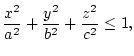
We saw how to find the absolute maximum and minmum for a function ![]() of two variables in
a given domain
of two variables in
a given domain ![]() (§15.6).
(§15.6).
Do problems §15.6: 1-6, 19-22, 27.
I will not be in my office in the morning tomorrow T, 10/12/04. Please schedule an appointment with me if you'd like to see me, or drop by at any other time.
We talked about the problem of finding the minimum or maximum of a function ![]() when
when
![]() is not free to take any values in the domain of definition of
is not free to take any values in the domain of definition of ![]() but it has to satisfy
some condition, which is usually given in the form
but it has to satisfy
some condition, which is usually given in the form
![]() .
Sometimes one can solve
.
Sometimes one can solve ![]() for one of the variables in
for one of the variables in ![]() and substitute the
resulting expression in
and substitute the
resulting expression in ![]() thus getting a problem of ordinary function extremization
without side conditions and in one variable less. We saw two such examples but this
method is most often inapplicable as it is not easy to solve
thus getting a problem of ordinary function extremization
without side conditions and in one variable less. We saw two such examples but this
method is most often inapplicable as it is not easy to solve
![]() for one of the variables,
especially if
for one of the variables,
especially if ![]() is a three-component vector and
is a three-component vector and ![]() is non-linear.
Even if possible the resulting expression for
is non-linear.
Even if possible the resulting expression for ![]() may be too complicated to work with.
may be too complicated to work with.
We then saw the method of Lagrange (or Lagrange multipliers as it is commonly known),
which allows one to solve the above problem by solving a, generally non-linear,
system of equations in the unknowns ![]() and
and ![]() , the latter being a auxiliary
variable which is not used except to help find the values of
, the latter being a auxiliary
variable which is not used except to help find the values of ![]() .
The system of equations is
.
The system of equations is
| 0 | |||
Some examples were discussed, and we will continue with this Friday.
We gave some more examples of the method of Lagrange multipliers and saw how it applies to the case of a function of three variable subject to two conditions.
Do problems §15.7: 1-4, 13, 15, 18-21, 23, 26
We remembered a few basic things about one variable integrals and how they are defined via sums corresponding to partitions of the intervals of integration. We then introduced the summation sign for both single and double sums and evaluated several examples.
Do problems §16.1: 1-4, 13-17.
We defined the integral of a function ![]() over a rectangle
over a rectangle ![]() via
lower and upper sums corresponding to partitions of
via
lower and upper sums corresponding to partitions of ![]() . We
evaluated, using the definition, only some simple integrals, and we then
saw how to extend this definition to arbitrary domains of integration.
Finally we saw some properties of the operation of integration which carry
over from the case of one-variable integration.
. We
evaluated, using the definition, only some simple integrals, and we then
saw how to extend this definition to arbitrary domains of integration.
Finally we saw some properties of the operation of integration which carry
over from the case of one-variable integration.
Do problems §16.2: 1, 2, 6, 7, 10, 11.
When a domain is such that all its intersections with lines parallel to the ![]() -axis are intervals,
and the set of
-axis are intervals,
and the set of ![]() -values used in the domain consititute an interval the domain is called of Type I
(and of Type II if the same properties hold with
-values used in the domain consititute an interval the domain is called of Type I
(and of Type II if the same properties hold with ![]() and
and ![]() reversed). For such a domain
we saw how to evaluate a double integral of a function as a single integral whose function to be integrated
is an integral itself.
reversed). For such a domain
we saw how to evaluate a double integral of a function as a single integral whose function to be integrated
is an integral itself.
Do problems §16.3: 1-6, 13, 14, 33, 34, 43, 46.
We saw how to evaluate a double integral using polar coordinates. The first task is to find
the domain ![]() in the
in the
![]() -plane which corresponds to the given domain
-plane which corresponds to the given domain
![]() (in the
(in the ![]() -plane). For example, if
-plane). For example, if ![]() is the unit disk in the cartesian plane
(the
is the unit disk in the cartesian plane
(the ![]() -plane) then
-plane) then ![]() is a rectangle in the
is a rectangle in the
![]() -plane defined by
-plane defined by
Do problems §16.4: 1, 2, 5, 6, 9, 10, 17-20, 23, 24.
The second test will be held after we finish Chapter 16. You'll be tested on chapters 15 and 16.
We covered the examples in §16.5. We saw how to compute the mass of a two-dimensional domain (a ``plate'') with variable density, and also how to compute its center of mass. We also saw how to compute the moment of inertia of a solid body (with variable density) rotating around a line in space. We specialized this to a rotating plate and evaluated some relevant double integrals. Last, we mentioned tha Parallel axis theorem. We did not have time to prove this (the proof is very simple and is in your book) but talked about what it means.
Do problems §16.5: 1-4, 11, 12, 14, 17, 25.
We saw briefly how triple integrals are defined (in a completely analogous way to oduble integrals,
so we did not insist much on §16.6) and proceeded to evaluate some triple integrals by repeated integration.
We also talked about the average fo a function ![]() over a domain
over a domain ![]() on which a density
function
on which a density
function
![]() is defined, and how this applies to the center of mass of a domain
with variable mass density.
is defined, and how this applies to the center of mass of a domain
with variable mass density.
Do problems: §16.7: 3-6, 11, 14-16, 21-22.
We computed some volumes and saw the following principle. Suppose we take a domain ![]() in
in
![]() and stretch it along the
and stretch it along the ![]() -axis by a factor of
-axis by a factor of ![]() to get a domain which we call
to get a domain which we call
![]() .
This means that a point
.
This means that a point
![]() if and only if
if and only if
![]() .
Then
.
Then
The second test will be held during the regular class hours on Monday, November 15, 2004. A review hour will be held on the previous Friday in class. You'll be tested on chapters 15 and 16 and the format of the test will be similar to the first one.
We showed how to compute a triple integral after first describing its domain of integration in cartesian coordinates.
Do problems: §16.8: 1-8, 11, 12, 17, 18, 25, 26.
Do the following problems in an hour with closed books (no calculators will be needed). In any test you write for this class you'll have to show all your work.
We introduced the spherical coordinate system and how to use it for evaluation
of triple integrals.
We saw several examples of how to transform the domain of integration from cartesian
to spherical coordinates and carry out the integration in spherical coordinates (the form
![]() becomes now
becomes now
![]() ).
In the last example we did (Example 3 in p. 1009 of your book) we got the wrong answer (0)
because teh range for
).
In the last example we did (Example 3 in p. 1009 of your book) we got the wrong answer (0)
because teh range for ![]() is not 0 to
is not 0 to ![]() , as we took it to be, but 0 to
, as we took it to be, but 0 to ![]() (remember
that
(remember
that ![]() is obvious from the equation of the surface).
is obvious from the equation of the surface).
Do problems §16.9: 1-4, 9-14, 16, 19, 20, 24, 26, 27.
Do the following problems in an hour with closed books (no calculators will be needed). In any test you write for this class you'll have to show all your work.
We saw the general procedure for evaluating a multiple (double or triple) integral
over a domain ![]() after first doing a change of variables. This is essentially
a way of parametrizing
after first doing a change of variables. This is essentially
a way of parametrizing ![]() using two or three variables (depending on the whether the
domain
using two or three variables (depending on the whether the
domain ![]() is in the plane or space) which run over a more convenient
domain
is in the plane or space) which run over a more convenient
domain ![]() . We say how to do this when
. We say how to do this when ![]() is a parallelogram (and we got a parametrization
with paramaters
is a parallelogram (and we got a parametrization
with paramaters ![]() and
and ![]() running through the rectangle
running through the rectangle
![]() )
and also in some other cases.
We also saw that the form
)
and also in some other cases.
We also saw that the form ![]() transforms into the form
transforms into the form
![]() (and similarly in three dimensions), where
(and similarly in three dimensions), where ![]() is the so-called
Jacobian determinant, which can be computed from the functions
is the so-called
Jacobian determinant, which can be computed from the functions ![]() and
and ![]() .
.
Do problems §16.10: 1-4, 8-10, 12-14, 19, 20, 25, 27, 29.
Please come to the review session on Friday prepared to ask questions.
Today we talked about some problems from chapters 15 and 16, as a preparation for Monday's test. The questions were chosen by the students.
Today we had our second test, during the usual class meeting. Here are the problems:
Someone forgot his calculator in class. It's in my office.
Date: Mon, 15 Nov 2004 13:30:34 -0500
From: Rhonda Mozingo <rmozingo@math.gatech.edu>
Subject: CIOS Survey Times

Please inform your students of the following CIOS schedule for the fall 2004 semester:

From Monday, November 22 -- 12:00 AM  until Friday, December 10 --  12:00 midnight course surveys will be on-line, 24/7
excluding Tuesdays Thursdays, and Saturdays from midnight to 3 AM when the system is down for maintenance.

Students may access the surveys:   www.coursesurvey.gatech.edu

If you or your students have any questions, please let me know.

Thank you,
Rhonda
You can find the results of the second test here.
We defined the line integrals of a vector field
![]() along a curve
along a curve ![]() given parametrically by
given parametrically by ![]() ,
,
![]() ,
as the expression
,
as the expression
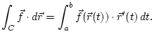
Do problems §17.1: 1-4, 7, 15, 16, 20, 21, 23, 25, 28-30.
This says that if a vector field ![]() is a gradient field, then a line integral of that
along a curve
is a gradient field, then a line integral of that
along a curve ![]() equals the value of
equals the value of ![]() (where
(where
![]() ) equals
) equals
![]() where
where ![]() and
and ![]() are the endpoints of
are the endpoints of ![]() . This is true in two and three dimensions,
and, in two dimensions, in order to decide if
. This is true in two and three dimensions,
and, in two dimensions, in order to decide if
![]() is a gradient field we need to verify
that
is a gradient field we need to verify
that ![]() when the domain
when the domain ![]() , where
, where ![]() is defined, is simply connected (i.e. connected
and with no ``holes'').
We saw several applications of that theorem as well as how to find
is defined, is simply connected (i.e. connected
and with no ``holes'').
We saw several applications of that theorem as well as how to find ![]() from
from ![]() .
.
Do problems §17.2: 1-4, 12, 13, 16, 17, 21, 22, 24-28.
We discussed kinetic energy and why its change is due to the work is done by the force field on the particle. Also we talked about conservative (gradient) fields and the potential function.
Do problems §17.3: 1-3, 6, 7.
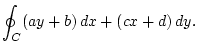
We saw an alternative way of writing the line integral
![]() as
as
![]() , where
, where
![]() .
We also saw the line integral w.r.t. arc-length, denoted by
.
We also saw the line integral w.r.t. arc-length, denoted by
![]() , where
, where
![]() is a scalar function.
is a scalar function.
Do problems §17.4: 2, 3, 5, 17, 18, 26, 27, 29, 30, 32, 36.
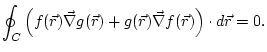
We stated Green's theorem. This expresses a line integral along a closed curve as a double integral over the interior of that curve. We proved this in the case when the domain if of Type I and of Type II and showed how one proves this if the domain is more general by cutting up the domain into a finite number of non-overlapping parts each of which is of both Type I and II. We also explained how to parametrize the boundary of a domain if that is not simply connected or even not connected (walk along the boundary in such a way that the domain is always on your left).
Do problems §17.5: 1, 2, 5, 6, 18-20, 26, 28, 30, 31.
My office hours this week will be held on Thursday, 9-11, instaed of Tuesday.
I just realized that the duration of the final exam (W, 12/8/04, at 11:30-2:20, in Skiles 271) is 2 hours and 50 minutes. So what I had told you about how many problems is not valid, as I thought the final was less than 2 hours long. You should expect at least 8 problems on the final. Probably half of these will cover Chapter 17.
We saw how to apply Green's formula to derive a formula for the area of a polygonal region
that has been described to us by the coordinates of its vertices. We also saw how to find an analogous
formula for the volume of the solid that arises if we rotate a polygonal region (which is part of the right half plane
![]() ) about the
) about the ![]() -axis.
-axis.
We'll have a review on Friday. Please come prepared to ask questions.
He had a very short discussion about the form of the final test and several procedural matters. We agreed that I'll try to grade all papers and set the grades by Thursday night and post them on the web. Then, we should settle all complaints by Friday.
There will most likely be 8 problems on the final exam four of which will cover Chapter 17 (through §17.5), and the remaining will cover Chapters 13-16.
Do the following problems in an hour with closed books (no calculators will be needed). In any test you write for this class you'll have to show all your work.
We had our final exam which lasted 2 hours and 20 minutes. Of the following 8 problems I ended up not taking problem 2 into account.


You can find the results of the final as well as the final letter grades here. I'll be in my office on Friday, 12/10/04, from 2:30 on for a couple of hours for questions and complaints.